Summary
Part of learning how to use any tool is exploring its strengths and weaknesses. I’m just starting to use the Python library Pandas, and my naïve use of it exposed a weakness that surprised me.
Background

I have a long list of objects, each with the properties “color” and “shape”. I want to count the frequency of each color/shape combination. A sample of what I’m trying to achieve could be represented in a grid like this –
       circle square star
blue        8     41   18
orange      5     33   25
red        53     64   58
At first I implemented this with a dictionary of collections.Counter instances where the top level dictionary is keyed by shape, like so –
import collections
SHAPES = ('square', 'circle', 'star', )
frequencies = {shape: collections.Counter() for shape in SHAPES}
Then I counted my frequencies using the code below. (For simplicity, assume that my objects are simple 2-tuples of (shape, color)).
for shape, color in all_my_objects:
    frequencies[shape][color] += 1
So far, so good.
Enter the Pandas
This looked to me like a perfect opportunity to use a Pandas DataFrame which would nicely support the operations I wanted to do after tallying the frequencies, like adding a column to represent the total number (sum) of instances of each color.
It was especially easy to try out a DataFrame because my counting loop ( for...all_my_objects) wouldn’t change, only the definition of frequencies. (Note that the code below requires I know in advance all the possible colors I can expect to see, which the Dict + Counter version does not. This isn’t a problem for me in my real-world application.)
import pandas as pd
frequencies = pd.DataFrame(columns=SHAPES, index=COLORS, data=0,
                           dtype='int')
for shape, color in all_my_objects:
    frequencies[shape][color] += 1
It Works, But…
Both versions of the code get the job done, but using the DataFrame as a frequency counter turned out to be astonishingly slow. A DataFrame is simply not optimized for repeatedly accessing individual cells as I do above.
How Slow is it?
To isolate the effect pandas was having on performance, I used Python’s timeit module to benchmark some simpler variations on this code. In the version of Python I’m using (3.6), the default number of iterations for each timeit test is 1 million.
First, I timed how long it takes to increment a simple variable, just to get a baseline.
Second, I timed how long it takes to increment a variable stored inside a collections.Counter inside a dict. This mimics the first version of my code (above) for a frequency counter. It’s more complex than the simple variable version because Python has to resolve two hash table references (one inside the dict, and one inside the Counter). I expected this to be slower, and it was.
Third, I timed how long it takes to increment one cell inside a 2×2 NumPy array. Since Pandas is built atop NumPy, this gives an idea of how the DataFrame’s backing store performs without Pandas involved.
Fourth, I timed how long it takes to increment one cell inside a 2×2 Pandas DataStore. This is what I had used in my real code.
Raw Benchmark Results
Here’s what timeit showed me. Sorry for the cramped formatting.
$ python
 Python 3.6.0 (v3.6.0:41df79263a11, Dec 22 2016, 17:23:13)
 [GCC 4.2.1 (Apple Inc. build 5666) (dot 3)] on darwin
 Type "help", "copyright", "credits" or "license" for more information.
 >>> import timeit
 >>> timeit.timeit('data += 1', setup='data=0')
 0.09242476700455882
 >>> timeit.timeit('data[0][0]+=1',setup='from collections import Counter;data={0:Counter()}')
 0.6838196019816678
 >>> timeit.timeit('data[0][0]+=1',setup='import numpy as np;data=np.zeros((2,2))')
 0.8909121589967981
 >>> timeit.timeit('data[0][0]+=1',setup='import pandas as pd;data=pd.DataFrame(data=[[0,0],[0,0]],dtype="int")')
 157.56428507200326
 >>>
Benchmark Results Summary
Here’s a summary of the results from above (decimals truncated at 3 digits). The rightmost column shows the results normalized so the fastest method (incrementing a simple variable) equals 1.
| Actual (seconds) | Normalized (seconds) | |
|---|---|---|
| Simple variable | 0.092 | 1 |
| Dict + Counter | 0.683 | 7.398 |
| Numpy 2D array | 0.890 | 9.639 |
| Pandas DataFrame | 157.564 | 1704.784 |
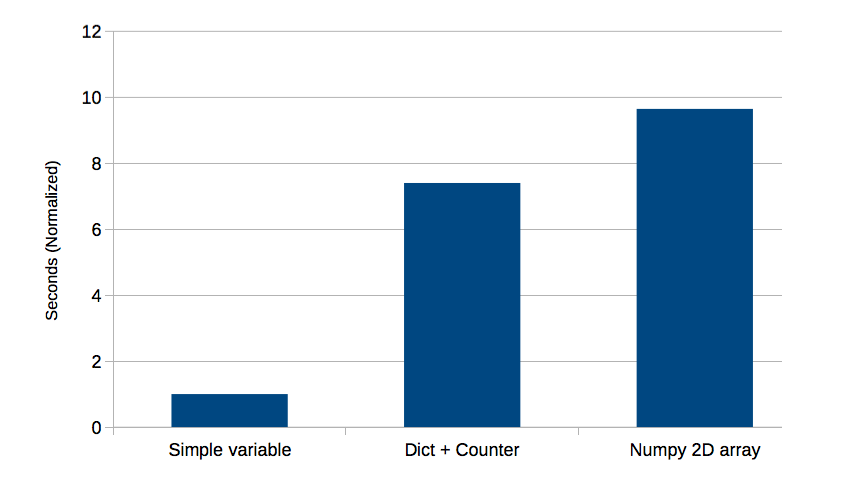
As you can see, resolving the index references in the middle two cases (Dict + Counter in one case, NumPy array indices in the other) slows things down, which should come as no surprise. The NumPy array is a little slower than the Dict + Counter.
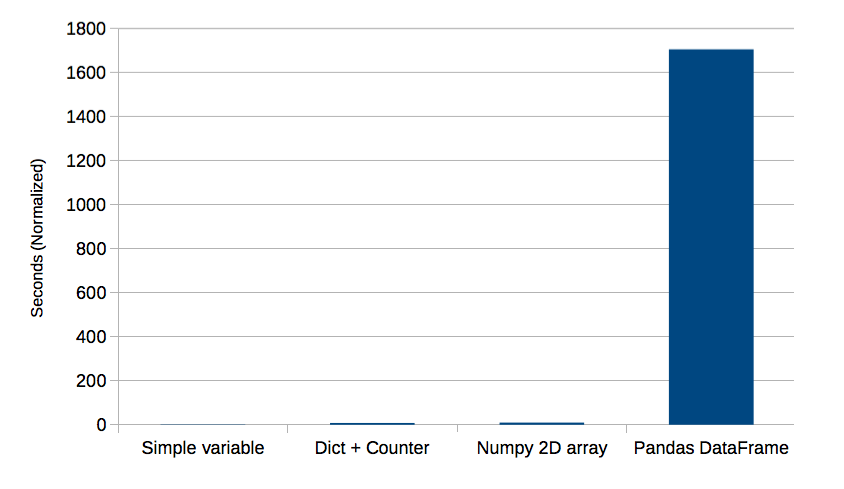
The DataFrame, however, is about 150 – 200 times slower than either of those two methods. Ouch!
I can’t really even give you a graph of all four of these methods together because the time consumed by the DataFrame throws the chart scale out of whack.
Here’s a bar chart of the first three methods –
Here’s a bar chart of all four –
Why Is My DataFrame Access So Slow?
One of the nice features of DataFrames is that they support dictionary-like labels for rows and columns. For instance, if I define my frequencies to look like this –
>>> SHAPES = ('square', 'circle', 'star', )
>>> COLORS = ('red', 'blue', 'orange')
>>> pd.DataFrame(columns=SHAPES, index=COLORS, data=0, dtype='int')
        square  circle  star
red          0       0     0
blue         0       0     0
orange       0       0     0
>>>
Then frequencies['square']['orange'] is a valid reference.
Not only that, DataFrames support a variety of indexing and slicing options including –
- A single label, e.g.
5or'a' - A list or array of labels
['a', 'b', 'c'] - A slice object with labels
'a':'f' - A boolean array
- A callable function with one argument
Here are those techniques applied in order to the frequencies DataFrame so you can see how they work –
>>> frequencies['star']
red       0
blue      0
orange    0
Name: star, dtype: int64
>>> frequencies[['square', 'star']]
        square  star
red          0     0
blue         0     0
orange       0     0
>>> frequencies['red':'blue']
      square  circle  star
red        0       0     0
blue       0       0     0
>>> frequencies[[True, False, True]]
        square  circle  star
red          0       0     0
orange       0       0     0
>>> frequencies[lambda x: 'star']
red       0
blue      0
orange    0
Name: star, dtype: int64
This flexibility has a price. Slicing (which is what is invoked by the square brackets) calls an object’s __getitem__() method. The parameter to __getitem__() is the whatever was inside the square brackets. A DataFrame’s __getitem__() has to figure out what the passed parameter represents. Determining whether the parameter is a label reference, a callable, a boolean array, or something else takes time.
If you look at the DataFrame’s __getitem__() implementation, you can see all the code that has to execute to resolve a reference. (I linked to the version of the code that was current when I wrote this in February of 2017. By the time you read this, the actual implementation may differ.) Not only does __getitem__() have a lot to do, but because I’m accessing a cell (rather than a whole row or column), there’s two slice operations, so __getitem__() gets invoked twice each time I increment my counter.
This explains why the DataFrame is so much slower than the other methods. The dictionary and Counter both only support key lookup in a hash table, and a NumPy array has far fewer slicing options than a DataFrame, so its __getitem__() implementation can be much simpler.
Better DataFrame Indexing?
DataFrames support a few methods that exist explicitly to support “fast” getting and setting of scalars. Those methods are .at() (for label lookups) and .iat() (for integer-based index lookups). It also provides get_value() and set_value(), but those methods are deprecated in the version I have (0.19.2).
“Fast” is how the Panda’s documentation describes these methods. Let’s use timeit to get some hard data. I’ll try at() and iat(); I’ll also try get_value()/set_value() even though they’re deprecated.
>>> timeit.timeit("data.at['red','square']+=1",setup="import pandas as pd;data=pd.DataFrame(columns=('square','circle','star'),index=('red','blue','orange'),data=0,dtype='int')")
36.33179204000044
>>> timeit.timeit('data.iat[0,0]+=1',setup='import pandas as pd;data=pd.DataFrame(data=[[0,0],[0,0]],dtype="int")')
42.01523362501757
>>> timeit.timeit('data.set_value(0,0,data.get_value(0,0)+1)',setup='import pandas as pd;data=pd.DataFrame(data=[[0,0],[0,0]],dtype="int")')
15.050199927005451
>>>
These methods are better, but they’re still pretty bad. Let’s put those numbers in context by comparing them to other techniques. This time, for normalized results, I’m going to use my Dict + Counter method as the baseline of 1 and compare all other methods to that. The row “DataFrame (naïve)” refers to naïve slicing, like frequencies[0][0].
| Actual (seconds) | Normalized (seconds) | |
|---|---|---|
| Dict + Counter | 0.683 | 1 |
| Numpy 2D array | 0.890 | 1.302 |
| DataFrame (get/set) | 15.050 | 22.009 |
| DataFrame (at) | 36.331 | 53.130 |
| DataFrame (iat) | 42.015 | 61.441 |
| DataFrame (naïve) | 157.564 | 230.417 |
The best I can do with a DataFrame uses deprecated methods, and is still over 20 times slower than the Dict + Counter. If I use non-deprecated methods, it’s over 50 times slower.
Workaround
I like label-based access to my frequency counters, I like the way I can manipulate data in a DataFrame (not shown here, but it’s useful in my real-world code), and I like speed. I don’t necessarily need blazing fast speed, I just don’t want slow.
I can have my cake and eat it too by combining methods. I do my counting with the Dict + Counter method, and use the result as initialization data to a DataFrame constructor.
SHAPES = ('square', 'circle', 'star', )
frequencies = {shape: collections.Counter() for shape in SHAPES}
for shape, color in all_my_objects:
    frequencies[shape][color] += 1

frequencies = pd.DataFrame(data=frequencies)
The frequencies DataFrame now looks something like this –
         circle square star
 blue         8     41   18
 orange       5     33   25
 red         53     64   58
The rows and columns appear in essentially random order; they’re ordered by whatever order Python returns the dict keys during DataFrame initialization. Getting them in a specific order is left as an exercise for the reader.
There’s one more detail to be aware of. If a particular (shape, color) combination doesn’t appear in my data, it will be represented by NaN in the DataFrame. They’re easy to set to 0 with frequencies.fillna(0).
Conclusion
What I was trying to do with Pandas – unfortunately, the very first thing I ever tried to do with it – didn’t play to its strengths. It didn’t break my code, but it slowed it down by a factor of ~1700. Since I had thousands of items to process, the difference was hard to overlook!
Pandas looks great for some things, and I expect I’ll continue using it. This was just a bump in the road, albeit an interesting one.